Spatial Statistics
"Everything is related to everything else, but near things are more related than distant things." — Tobler's First Law of Geography
Motivations for Our Spatial Statistics Research:
To study real phenomena, one might ideally take measurements at infinitely many spatial coordinates. This indexed collection of measurements is what we call a spatial field. In practice, however, dense measurements are often infeasible or impossible to obtain (for example, subsurface topography). Instead, we model the field as a random process. An ideal random field captures the essential structure of a complicated phenomenon using only a few physically meaningful parameters. We assume the field is Gaussian because Gaussian fields are fully characterized by their first- and second-order statistics. Of particular importance are the second-order statistics, since they describe correlation structure in space.
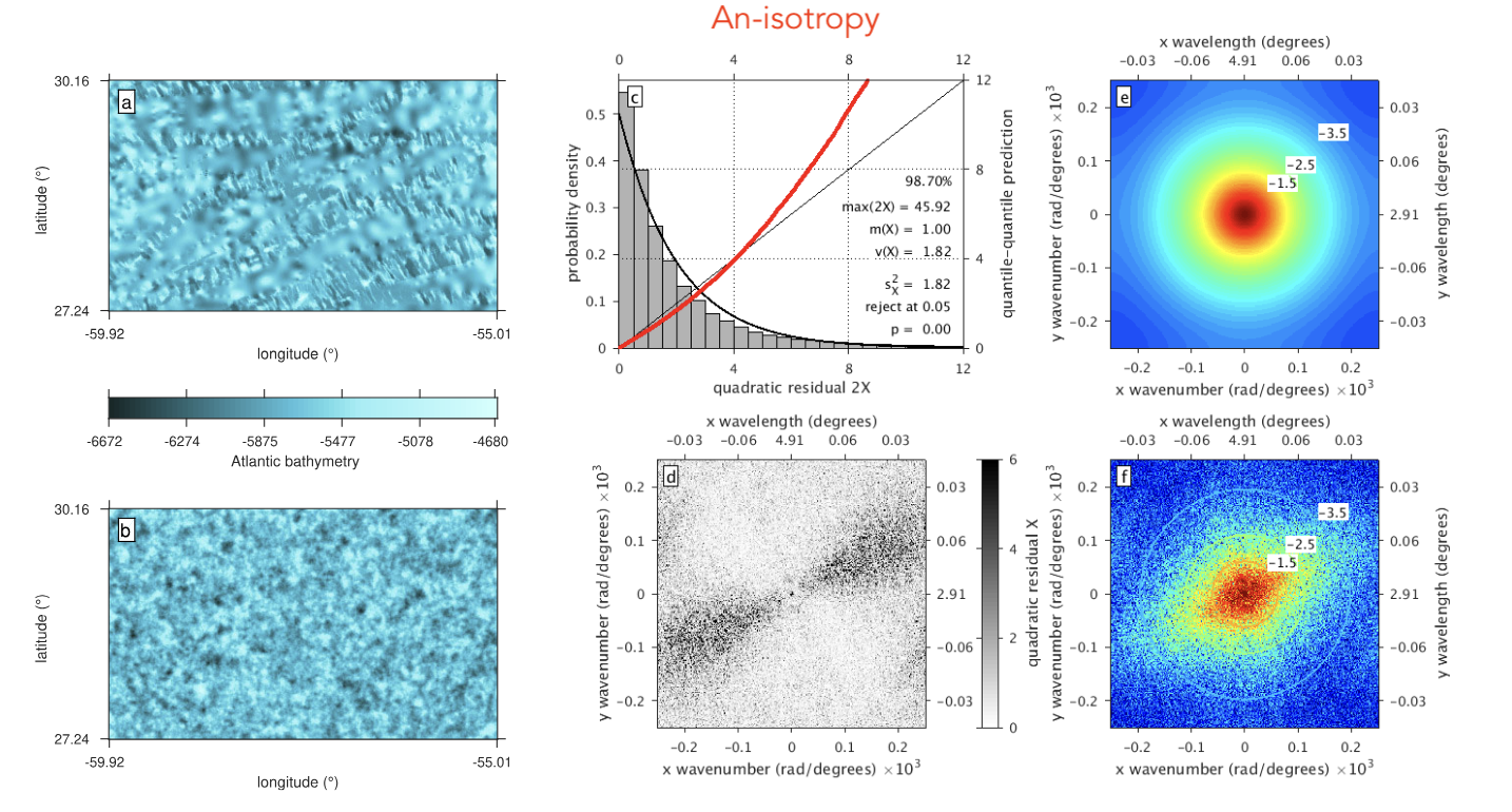
Spatial correlations can be interpreted in terms of oscillatory structure. This motivates Fourier analysis and the Wiener–Khinchin relationship between covariance and spectrum. We additionally assume isotropy as the null hypothesis. We use a zero mean and a Matérn covariance model. We choose Matérn covariance because its parameters —variance, smoothness, and range— are physically meaningful.
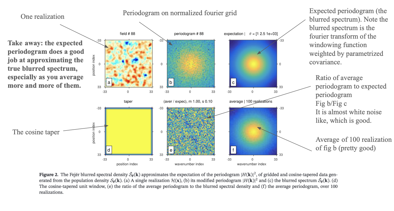
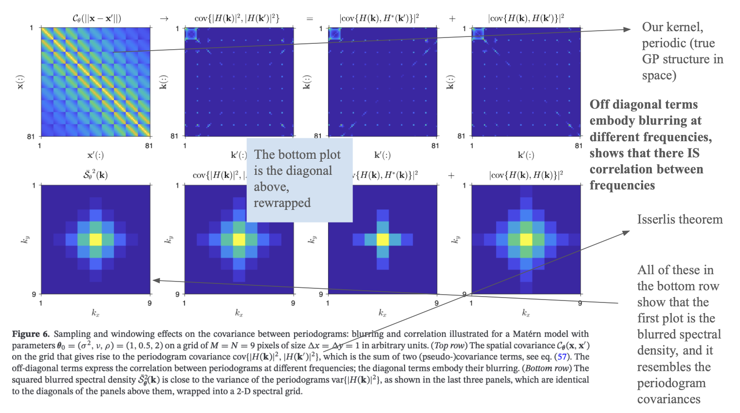
Although the spatial and spectral domains contain equivalent information, the spectral domain is often computationally advantageous because it approximately diagonalizes the problem. For an infinite stationary field, different wavenumbers are uncorrelated in the spectral domain. The major complication is that real observations are finite and sampled. Finite spatial windows introduce spectral leakage/blurring (“boundary effects”) and induce correlations between nearby wavenumbers. Increasing the spatial domain helps reduce these effects because larger windows better capture long-range correlations and reduce spectral leakage.
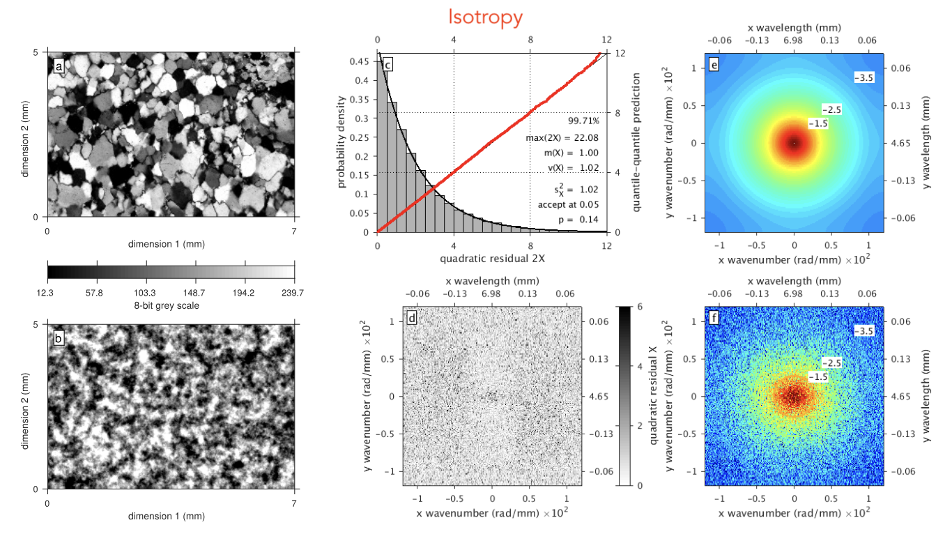
To make likelihood-based inference computationally feasible, we often use the Whittle likelihood, which approximates the full covariance likelihood in the spectral domain. To assess parameter resolution and uncertainty, we study quantities such as the score function, Hessian, Fisher information matrix, and residual diagnostics (which will follow a chi-squared with 2 degrees of freedom due to the quadratic form of the likelihood). The Fisher information matrix measures how sensitive the likelihood is to changes in model parameters. Larger values generally indicate parameters that are better resolved by the data.
Key Spatial Questions:
- It gives us information about spatial relationships
- It allows us to model random fields (stochastic processes in multiple dimensions)
- It can be applied to a number of problems (interpolation, extrapolation, simulation, modeling, growing-domain, etc.)
Spatial statistics is the study of an indexed family of random variables, $Z(\textbf{s})$. A random variable can be thought of as a mapping from outcomes to numbers. The Z notation for a random variable is just a nod to the fact that we have the ability to work with complex values. The "index" refers to the spatial vector s that can live in any dimension. For instance, a cartesian map with 5 points on it will be represented as $(\textbf{s}_1,\textbf{s}_2,\textbf{s}_3,\textbf{s}_4,\textbf{s}_5)$ where each $\textbf{s}_i=(\phi_i,\lambda_i)$ for latitude and longitude. Lastly, something to be aware of is that functions of random variables are random variables themselves.
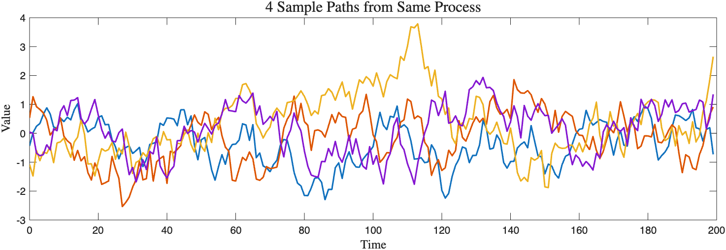
A Gaussian process is a generalization of a random variable. More specifically, it is a distribution over functions. Instead of each "draw" or "realization" being a number, each realization is an entire function called a sample path. Four 1D sample paths in the time/spatial domain are pictured below, each generated with the same mean and covariance structure.
The covariance kernel/matrix/function provides the underlying structure of the field (tunable through parameters such as correlation length or variance). Choosing a covariance structure can be a bit arbitrary at times. In general, you want to model it off of the properties you observe in your time series/data (is it periodic? stationary? smooth?...). I refer the interested reader to the Kernel Cookbook . The only rules for choosing a kernel is that it has to be symmetric and positive semi-definite. To incorporate randomness, you are essentially transforming white noise with the covariance kernel:
$C(t,t') = LL^T$
${cov}(Lz)=L^Tcov(z)L=LIL^T=LL^T=C(t,t')$
One can imagine that if you sample more and more, a distribution over the sample paths will emerge. That is called your latent function distribution, which I like to think about as the background function. We choose a Gaussian distribution because it is uniquely determined by only two measurements (mean and covariance), is closed under conditioning, and is closed under marginalization.
- A Gaussian process is completely determined by its first and second moments
- All finite subsets of Gaussian processes must be jointly Gaussian
- Covariance controls structure
- More data reduces uncertainty
- Conditioning updates beliefs
Convergence analysis allows us to make statements about long-term asymptotics of a sequence of random variables $X_n$. This is amazing because it can tell us if random events settle into patterns (whether about the mean, probability, or distribution).
In probability theory, there exist three types of convergence of sequences of random variables (ordered here from weakest to strongest):
- Convergence in distribution (law): $F_{X_n}(x)\rightarrow F_X(x)$ (think: the histograms match)
- If you roll a fair die many, many times, you'd expect the histogram to converge to the uniform distribution.
- Convergence in probability: $P(|X_n-X|>\epsilon)\rightarrow0$ (think: they are close)
- If you were to plot the height of more and more people, the true mean human height would emerge.
- Almost sure convergence: $P(X_n\rightarrow X)=1$ (think: we know how the sample paths will converge)
- If you studied how much a specific animal eats per day, that will fluctuate. But one day, you will be almost sure it will be 0.
The CLT and WLLN both study the same object, namely the sample mean $\bar X_n=\frac1N\sum X_i$, but ask two different questions about it:
- CLT: What is the long-term distribution of the sample mean? $ \frac{\sqrt n}{\sigma} (\bar X_n-\mu) \rightarrow N(0,1) $
- WLLN: What does the sample mean get closer and closer to? $ \bar X_n \rightarrow \mu $
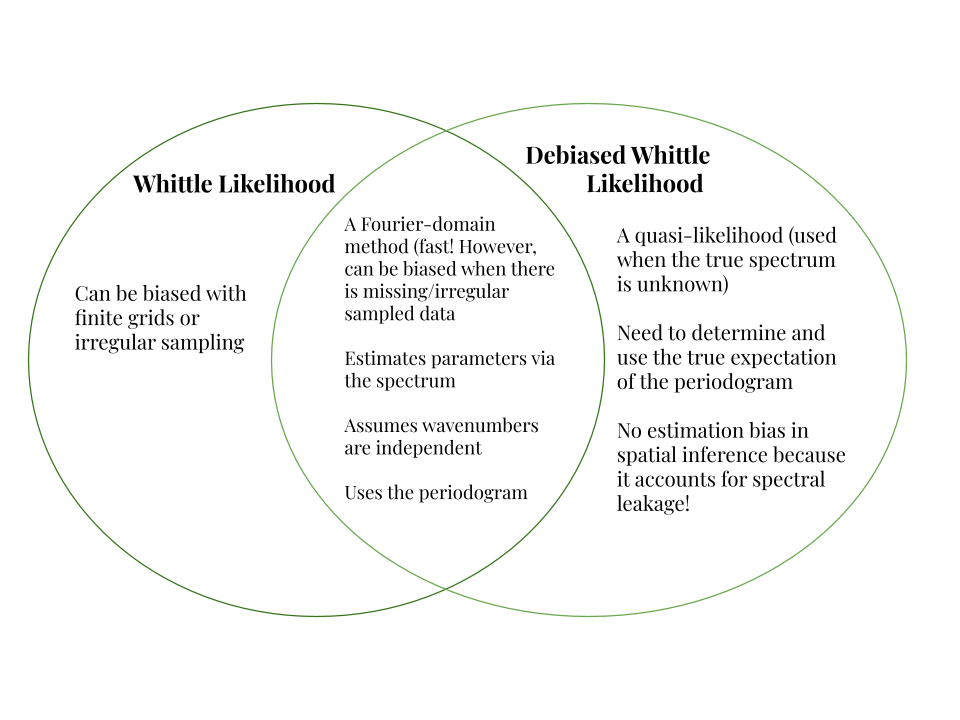 The debiased Whittle likelihood is given by: